Exercise 3 - Visualize Data with the Genome Data Viewer

Background

What is the Genome Data Viewer?

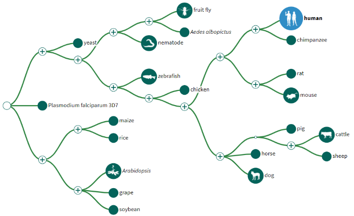
NCBI’s Genome Data Viewer (GDV) is a genome “browser” which supports the visualization of genetic data mapped against any of >1500 NCBI curated/annotated eukaryotic reference genomes.  https://www.ncbi.nlm.nih.gov/genome/gdv/

Data is visualized in "tracks".

• You can include gene/feature annotations, sequence coverage, GWAS data, and more!
• You can mix/match between your own tracks and NCBI/partner proivded ones!
  
  

Objective 3 Goals

Computational

• Access and navigate the GDV
• Upload custom data tracks to GDV
• Parse biological meaning from alignment results
• Use NCBI track data to find known clinical relevance

Case Study

• Identify structural changes between patient DNA and reference sequence to identify possible deletions in BBS related gene
• Use NCBI dbVar data to match results to known structural variants

Setup the Genome Data Viewer

1) Open a new tab in your web browser and go to https://ncbi.nlm.nih.gov/genome/gdv/

2) Make sure the Human is selected from the tree on the left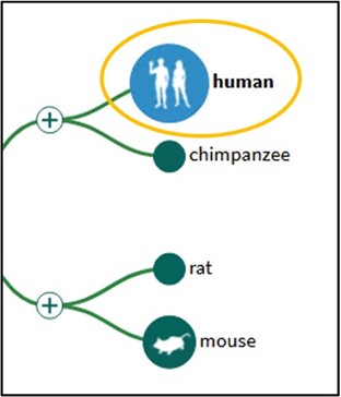



3) Scroll to the bottom of the page and click on the 7th Chromosome image to load the Genome Data Viewer on the human reference genome’s 7th chromosome



4) The GDV page comes pre-loaded with several tracks aligned against the chromosome. Most of these are not useful to us today, so we can use the red X buttons in the top right corner of each track to delete them. Do this for every track except the top one. This top track shows every gene and its position on the chromosome.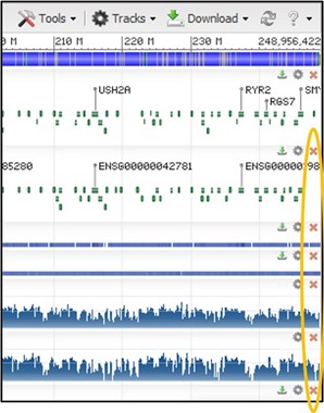

NOTE: There are LOTS of NCBI-offered tracks you can upload ato compare against your own data. To learn more about them click the little gear at the bottom of the viewer page: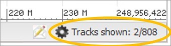

Importing Our Data

1) Click on User Data and Track Hubs on the left side of the screen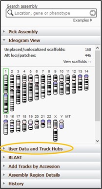

2) Click the Options pulldown menu and click Add Remote Files…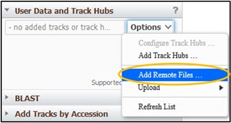

3) Navigate back to your S3 bucket tab and click on the SRR6314034.sorted.bam file to open up the details for the file

4) On the new page, click the “Copy” button next to the Object URL to copy the URL path to the file to your clipboard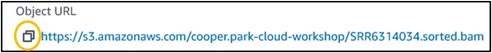

5) Go back to your GDV tab and paste the link into the URL box. Next, add a familiar name like Child to the Name box to help us identify the track later. Then click Add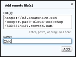

6) This track is showing all of the results of magicBLAST in a “pile-up” view. This is basically one long histogram plot where a taller bar represents a region of the chromosome where more reads from the sample aligned to. Because our sequences are specific to a single gene in the chromosome, but our current view is showing the entire chromosome, the pile-up view may look a little bland.
Try to find the region of the chromosome that our reads aligned to: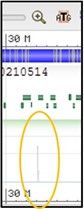

7) Use the scale bar at the top of the viewer and click-and-drag across the section where our reads aligned to highlight it. Then use the pop-up menu to click Zoom On Range

8) Repeat step 7 using the new view to refine the range again if the view didn’t change very much.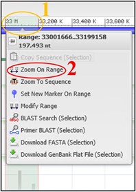

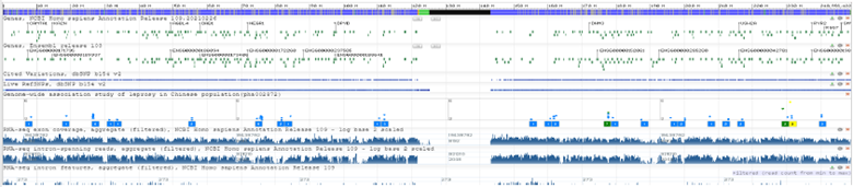
9) Your view should now see the track similar to the screenshot below. If you don’t see the mess of red lines below the thick black bar, that’s okay! We will turn it off next anyway.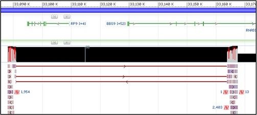

NOTE: The tracks may be slightly different depending on how you have zoomed in. As long as you can see the image above somewhere on your screen you are doing great!

10) Those red lines underneath the thick black box are showing how each individual sequence read aligned to the reference sequence. This particular view isn’t very helpful to us, so let’s turn it off.

NOTE: If you can’t see these lines, that’s great! You can skip Steps 15 & 16

11) Click the little gear in the top right corner of our Child track to open its settings.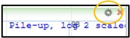

12) On this new menu page, change the “Alignment Display” to “Packed” and then click Accept. You can change many other settings here as well, but I’ll leave that up to you to explore outside of this workshop.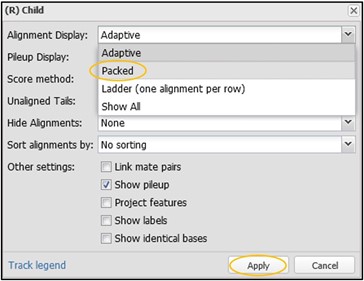

Now that we can see the range a bit better, let’s break down what each of these colors represent in the pile-up view:

• Grey – This is the standard “bar” for the pile-up view. The taller this bar is in a particular region, the greater the coverage is from the mapped reads.
• Red – These are locations in the genome where reads mapped, but with mismatches in the nucleotide sequence compared to the reference sequence.
• Black – These are gaps that exist in the read alignment to the reference genome (i.e., the reads only have a nucleotide sequence that covers before/after the large black chunk).

If you want to explore the pile-up view a bit more, try using the buttons in the toolbar just above the numeric range to navigate the assembly. Hold your mouse over the button for a description of what they can do!

Adding NCBI Data

1) Click the Tracks button in the bottom right corner of the viewer panel to open the Configure Page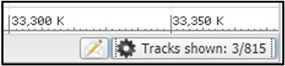



2) Click on the Variation tab and scroll way WAY down to the dbVar category. Then click the checkbox next to dbVar Pathogenic Clinical Structural Variants then click Configure in the bottom right corner of the page.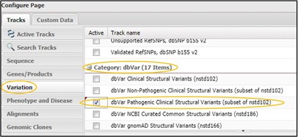



3) You should now have a new structural variants track loaded into the viewer. This track shows the region of the genome where each variant is found. Blue variants are caused by an insertion in this region, while Red variants are caused by a deletion. Because our alignment suggests a deletion, we want to focus on the red variants.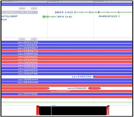



4) Next, zoom in on the right-half of our aligned region in the child track like the screenshot below. We want to look closely at the BBS9 gene to find structural variants that overlap with this region.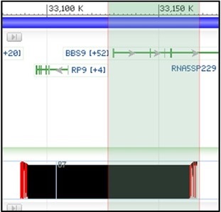



5) Obviously, there are a LOT of variants that overlap in this region. However, our concern is only about our sequenced region of the gene. Variants which extend beyond our sequenced region are less likely to be relevant for us. So rather than just aimlessly checking every red variant, lets look only for variants that start or stop within our deletion.

Oh… there’s just one? Let’s check that one then.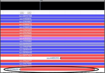



6) Mouse over the variant nsv1398255 to get a new pop-up menu and select the dbVar link at the bottom of it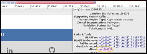



7) On the dbVar page, navigate to the Clinical Assertions panel to see which clinical conditions have been associated with this deletion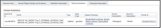



8) Just as we suspected! This region is associated with Bardet-biedl syndrome. If we wanted to, we could click on the phenotype and explore more about the condition. But that is something you need to explore on your own, because this is the end of the worksheet!

Page 1 of 1